[1]:

import atmPy.aerosols.size_distribution.sizedistribution as atmsd

[30]:

import warnings
warnings.simplefilter('ignore')

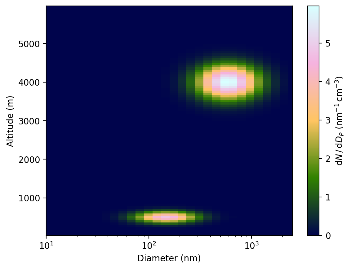
SizeDist_LS - a layer series (aka vertical profile) of size distributions

SizeDist_TS is a subclass of SizeDist with all its properties methods, etc. Here we will mostly focus on what is unique to the SizeDist_TS class.

Create instance

simulate a sizedistribution

[31]:

sd = atmsd.simulate_sizedistribution_layerseries(diameter=[10, 2500],
                                                numberOfDiameters=30,
                                                heightlimits=[0, 6000],
                                                noOflayers=50,
                                                layerHeight=[500.0, 4000.0],
                                                layerThickness=[100.0, 300.0],
                                                layerDensity=[1000.0, 5000.0],
                                                layerModecenter=[200.0, 800.0],
                                                widthOfAerosolMode=0.2,)

format your own data

data should have a similar structure as below. However, column names are not required as they are calculated based on bins

[3]:

sd.data

[3]:

bincenters	11.048638	13.365842	16.169028	19.560119	23.662416	28.625078	34.628546	41.891108	50.676829	61.305159	...	411.502887	497.806397	602.210134	728.510216	881.298909	1066.131608	1289.728823	1560.220544	1887.441843	2283.290476
30.0	3.052113e-12	3.131145e-11	2.707518e-10	1.973355e-09	1.212285e-08	6.277254e-08	2.739684e-07	1.007852e-06	3.125064e-06	8.167451e-06	...	1.003399e-05	4.000585e-06	1.344432e-06	3.808201e-07	9.092150e-08	1.829696e-08	3.103537e-09	4.437113e-10	5.346995e-11	5.431060e-12
90.0	4.276988e-11	4.387737e-10	3.794100e-09	2.765302e-08	1.698799e-07	8.796444e-07	3.839175e-06	1.412324e-05	4.379215e-05	1.144522e-04	...	1.406084e-04	5.606101e-05	1.883980e-05	5.336510e-06	1.274101e-06	2.563990e-07	4.349049e-08	6.217817e-09	7.492852e-10	7.610656e-11
150.0	4.181474e-10	4.289750e-09	3.709370e-08	2.703547e-07	1.660862e-06	8.600002e-06	3.753438e-05	1.380784e-04	4.281419e-04	1.118962e-03	...	1.374683e-03	5.480906e-04	1.841907e-04	5.217335e-05	1.245648e-05	2.506731e-06	4.251926e-07	6.078961e-08	7.325522e-09	7.440695e-10
210.0	2.852166e-09	2.926021e-08	2.530146e-07	1.844078e-06	1.132867e-05	5.866026e-05	2.560205e-04	9.418269e-04	2.920338e-03	7.632395e-03	...	9.376656e-03	3.738503e-03	1.256357e-03	3.558723e-04	8.496515e-05	1.709831e-05	2.900221e-06	4.146434e-07	4.996708e-08	5.075267e-09
270.0	1.357295e-08	1.392441e-07	1.204051e-06	8.775639e-06	5.391110e-05	2.791537e-04	1.218356e-03	4.481986e-03	1.389737e-02	3.632120e-02	...	4.462183e-02	1.779087e-02	5.978779e-03	1.693533e-03	4.043340e-04	8.136780e-05	1.380163e-05	1.973214e-06	2.377844e-07	2.415229e-08
...	...	...	...	...	...	...	...	...	...	...	...	...	...	...	...	...	...	...	...	...	...
5730.0	3.630329e-24	1.292883e-22	3.880953e-21	9.819357e-20	2.094080e-18	3.764170e-17	5.703098e-16	7.283131e-15	7.839547e-14	7.112618e-13	...	2.220879e-07	3.073871e-07	3.586013e-07	3.526174e-07	2.922545e-07	2.041664e-07	1.202190e-07	5.966609e-08	2.496018e-08	8.801028e-09
5790.0	1.122985e-24	3.999329e-23	1.200511e-21	3.037462e-20	6.477705e-19	1.164386e-17	1.764163e-16	2.252921e-15	2.425039e-14	2.200175e-13	...	6.869938e-08	9.508530e-08	1.109276e-07	1.090766e-07	9.040428e-08	6.315564e-08	3.718784e-08	1.845676e-08	7.721035e-09	2.722458e-09
5850.0	3.337566e-25	1.188620e-23	3.567978e-22	9.027487e-21	1.925206e-19	3.460614e-18	5.243179e-17	6.695792e-16	7.207337e-15	6.539030e-14	...	2.041779e-08	2.825982e-08	3.296823e-08	3.241810e-08	2.686860e-08	1.877017e-08	1.105241e-08	5.485440e-09	2.294730e-09	8.091280e-10
5910.0	9.530465e-26	3.394122e-24	1.018841e-22	2.577811e-21	5.497452e-20	9.881830e-19	1.497197e-17	1.911992e-16	2.058065e-15	1.867229e-14	...	5.830329e-09	8.069631e-09	9.414124e-09	9.257032e-09	7.672365e-09	5.359848e-09	3.156031e-09	1.566375e-09	6.552632e-10	2.310476e-10
5970.0	2.614728e-26	9.311935e-25	2.795239e-23	7.072347e-22	1.508252e-20	2.711127e-19	4.107631e-18	5.245642e-17	5.646398e-16	5.122831e-15	...	1.599578e-09	2.213941e-09	2.582809e-09	2.539711e-09	2.104950e-09	1.470500e-09	8.658720e-10	4.297423e-10	1.797746e-10	6.338901e-11

100 rows × 29 columns

bins are the binedges. For an example of how they should be formatted look again to the sizedistribution generated above

[4]:

sd.bins

[4]:

array([  10.        ,   12.09727592,   14.63440848,   17.70364774,
         21.41659115,   25.90824126,   31.34191432,   37.91517855,
         45.86703767,   55.48662105,   67.1236965 ,   81.20138776,
         98.23155932,  118.83342776,  143.75607647,  173.90569229,
        210.37851445,  254.50069379,  307.87651158,  372.44671113,
        450.55906317,  545.05373075,  659.36653747,  797.65389392,
        964.9439247 , 1167.31929089, 1412.1383554 , 1708.3027329 ,
       2066.58095226, 2500.        ])

To see options for the distType argument see help file. This is what our generated was:

[5]:

sd.distributionType

[5]:

'dNdDp'

[8]:

sd.layerbounderies

[8]:

array([[   0.,   60.],
       [  60.,  120.],
       [ 120.,  180.],
       [ 180.,  240.],
       [ 240.,  300.],
       [ 300.,  360.],
       [ 360.,  420.],
       [ 420.,  480.],
       [ 480.,  540.],
       [ 540.,  600.],
       [ 600.,  660.],
       [ 660.,  720.],
       [ 720.,  780.],
       [ 780.,  840.],
       [ 840.,  900.],
       [ 900.,  960.],
       [ 960., 1020.],
       [1020., 1080.],
       [1080., 1140.],
       [1140., 1200.],
       [1200., 1260.],
       [1260., 1320.],
       [1320., 1380.],
       [1380., 1440.],
       [1440., 1500.],
       [1500., 1560.],
       [1560., 1620.],
       [1620., 1680.],
       [1680., 1740.],
       [1740., 1800.],
       [1800., 1860.],
       [1860., 1920.],
       [1920., 1980.],
       [1980., 2040.],
       [2040., 2100.],
       [2100., 2160.],
       [2160., 2220.],
       [2220., 2280.],
       [2280., 2340.],
       [2340., 2400.],
       [2400., 2460.],
       [2460., 2520.],
       [2520., 2580.],
       [2580., 2640.],
       [2640., 2700.],
       [2700., 2760.],
       [2760., 2820.],
       [2820., 2880.],
       [2880., 2940.],
       [2940., 3000.],
       [3000., 3060.],
       [3060., 3120.],
       [3120., 3180.],
       [3180., 3240.],
       [3240., 3300.],
       [3300., 3360.],
       [3360., 3420.],
       [3420., 3480.],
       [3480., 3540.],
       [3540., 3600.],
       [3600., 3660.],
       [3660., 3720.],
       [3720., 3780.],
       [3780., 3840.],
       [3840., 3900.],
       [3900., 3960.],
       [3960., 4020.],
       [4020., 4080.],
       [4080., 4140.],
       [4140., 4200.],
       [4200., 4260.],
       [4260., 4320.],
       [4320., 4380.],
       [4380., 4440.],
       [4440., 4500.],
       [4500., 4560.],
       [4560., 4620.],
       [4620., 4680.],
       [4680., 4740.],
       [4740., 4800.],
       [4800., 4860.],
       [4860., 4920.],
       [4920., 4980.],
       [4980., 5040.],
       [5040., 5100.],
       [5100., 5160.],
       [5160., 5220.],
       [5220., 5280.],
       [5280., 5340.],
       [5340., 5400.],
       [5400., 5460.],
       [5460., 5520.],
       [5520., 5580.],
       [5580., 5640.],
       [5640., 5700.],
       [5700., 5760.],
       [5760., 5820.],
       [5820., 5880.],
       [5880., 5940.],
       [5940., 6000.]])

create the instance

[9]:

sdc = atmsd.SizeDist_LS(sd.data, sd.bins, sd.distributionType, sd.layerbounderies)

Methods

Plotting

[10]:

sd.plot()

[10]:

(<Figure size 1280x960 with 2 Axes>,
 <Axes: xlabel='Diameter (nm)', ylabel='Altitude (m)'>,
 <matplotlib.collections.QuadMesh at 0x7efdf7dfcd60>,
 <matplotlib.colorbar.Colorbar at 0x7efdf7c06470>)

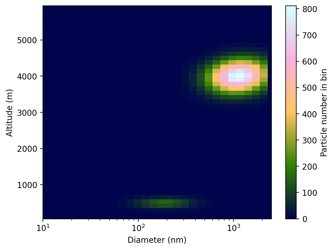
hygroscopic growth and optical properties

The difference to hygroscopic growth and optical properties of the SizeDist instance is that you can let the RH and refractive index change over time.

GOTCHA you can loose particles when applying growth!!! See help of sd.grow_sizedistribution function! There are functions that extrapolate size distributions assuming normal distributions. Consider using those.

[43]:

reload(atmsd.hygroscopicity)
reload(atmsd.optical_properties)
reload(atmsd)

[43]:

<module 'atmPy.aerosols.size_distribution.sizedistribution' from '/export/htelg/prog/atm-py/atmPy/aerosols/size_distribution/sizedistribution.py'>

[44]:

sd = atmsd.SizeDist_LS(sd.data, sd.bins, sd.distributionType, sd.layerbounderies)

[45]:

sd.optical_properties.parameters.refractive_index = 1.5
sd.optical_properties.parameters.wavelength = 500

[46]:

rh = pd.DataFrame(index = sd.data.index, columns=['RH'], dtype=float)
rh.RH.iloc[[0,-1]] = [0,95]
rh = rh.interpolate()
rh.shape

[46]:

(50, 1)

[47]:

sd.hygroscopicity.parameters.kappa = 1.5
sd.hygroscopicity.parameters.RH = rh

[48]:

sd.hygroscopicity.grown_size_distribution.plot()

[48]:

(<Figure size 1280x960 with 2 Axes>,
 <Axes: xlabel='Diameter (nm)', ylabel='Altitude (m)'>,
 <matplotlib.collections.QuadMesh at 0x7efdec2d9060>,
 <matplotlib.colorbar.Colorbar at 0x7efde9db9900>)

[49]:

a = sd.optical_properties.scattering_coeff.plot()
sd.hygroscopicity.grown_size_distribution.optical_properties.scattering_coeff.plot(ax = a)

[49]:

<Axes: ylabel='Altitude'>

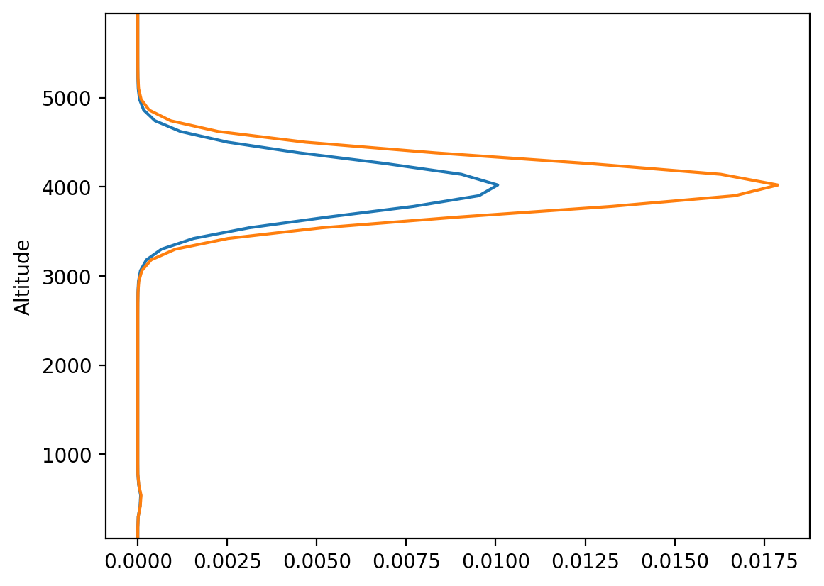
Note, the refractive index of the hygroscopically grown size distribution is changing and approaches that of water.

[50]:

sd.hygroscopicity.grown_size_distribution.optical_properties.parameters

[50]:

asphericity      :  1
mie_result       :  None
refractive_index :          index_of_refraction
60.0               1.500000
180.0              1.495104
300.0              1.490300
420.0              1.485588
540.0              1.480963
660.0              1.476423
780.0              1.471967
900.0              1.467592
1020.0             1.463295
1140.0             1.459076
1260.0             1.454930
1380.0             1.450858
1500.0             1.446856
1620.0             1.442923
1740.0             1.439057
1860.0             1.435256
1980.0             1.431519
2100.0             1.427845
2220.0             1.424231
2340.0             1.420676
2460.0             1.417179
2580.0             1.413739
2700.0             1.410353
2820.0             1.407021
2940.0             1.403742
3060.0             1.400513
3180.0             1.397335
3300.0             1.394205
3420.0             1.391124
3540.0             1.388088
3660.0             1.385099
3780.0             1.382154
3900.0             1.379252
4020.0             1.376394
4140.0             1.373576
4260.0             1.370800
4380.0             1.368064
4500.0             1.365366
4620.0             1.362707
4740.0             1.360085
4860.0             1.357500
4980.0             1.354951
5100.0             1.352437
5220.0             1.349957
5340.0             1.347511
5460.0             1.345098
5580.0             1.342717
5700.0             1.340368
5820.0             1.338050
5940.0             1.335763
wavelength       :  500

AOD (aerosol optical depth)

A vertical profile of aerosol optical properties can be integrated to the AOD

[52]:

sd.optical_properties.aod, sd.hygroscopicity.grown_size_distribution.optical_properties.aod

[52]:

(7.599809165410463, 13.401056561321452)

[ ]: