[1]:
import atmPy.aerosols.size_distribution.sizedistribution as atmsd
SizeDist (a single size distribution)
Create instance
simulate a sizedistribution
[8]:
sd = atmsd.simulate_sizedistribution(diameter=[10, 2500],
                                    numberOfDiameters=100,
                                    centerOfAerosolMode=200,
                                    widthOfAerosolMode=0.2,
                                    numberOfParticsInMode=1000,)
format your own data
[5]:
atmsd.SizeDist(data, bins, distType)
data should have a similar structure as below. However, column names are not required as they are calculated based on bins
[11]:
sd.data
[11]:
| bincenters | 10.286785 | 10.876803 | 11.500663 | 12.160306 | 12.857784 | 13.595267 | 14.375049 | 15.199558 | 16.071358 | 16.993162 | ... | 1472.324349 | 1556.772354 | 1646.064038 | 1740.477219 | 1840.305650 | 1945.859933 | 2057.468486 | 2175.478563 | 2300.257336 | 2432.193036 |
|---|---|---|---|---|---|---|---|---|---|---|---|---|---|---|---|---|---|---|---|---|---|
| 0 | 8.067904e-08 | 1.653171e-07 | 3.338144e-07 | 6.642360e-07 | 0.000001 | 0.000003 | 0.000005 | 0.000009 | 0.000017 | 0.00003 | ... | 0.000049 | 0.000027 | 0.000015 | 0.000008 | 0.000004 | 0.000002 | 0.000001 | 5.883500e-07 | 2.949072e-07 | 1.456683e-07 |
1 rows × 99 columns
bins are the binedges. For an example of how they should be formatted look again to the sizedistribution generated above
[12]:
sd.bins
[12]:
array([  10.        ,   10.57356931,   11.18003679,   11.82128938,
         12.49932225,   13.21624501,   13.97428826,   14.77581054,
         15.62330568,   16.51941053,   17.46691322,   18.46876174,
         19.52807323,   20.64814357,   21.8324577 ,   23.08470046,
         24.40876803,   25.80878004,   27.28909244,   28.85431102,
         30.50930573,   32.25922586,   34.10951604,   36.06593318,
         38.1345644 ,   40.32184597,   42.63458328,   45.07997211,
         47.66562094,   50.39957465,   53.29033955,   56.34690986,
         59.57879565,   62.99605249,   66.6093127 ,   70.42981842,
         74.46945662,   78.74079607,   83.25712644,   88.03249966,
         93.08177363,   98.42065845,  104.06576532,  110.03465819,
        116.34590844,  123.01915263,  130.07515362,  137.53586517,
        145.42450023,  153.76560319,  162.58512621,  171.91050999,
        181.77076917,  192.19658255,  203.22038858,  214.87648629,
        227.20114199,  240.23270211,  254.01171251,  268.58104466,
        283.98602898,  300.27459591,  317.49742505,  335.7081028 ,
        354.96328913,  375.32289384,  396.85026299,  419.61237596,
        443.68005385,  469.12817988,  496.0359323 ,  524.48703081,
        554.56999699,  586.37842978,  620.01129664,  655.57324151,
        693.17491038,  732.93329556,  774.97209967,  819.42212055,
        866.42165819,  916.11694505,  968.66260102, 1024.22211453,
       1082.9683512 , 1145.08409168, 1210.76260037, 1280.20822673,
       1353.63704105, 1431.27750677, 1513.37119129, 1600.17351757,
       1691.95455884, 1788.99987893, 1891.6114207 , 2000.10844554,
       2114.8285267 , 2236.12859958, 2364.38607231, 2500.        ])
To see options for the distType argument see help file. This is what our generated was:
[13]:
sd.distributionType
[13]:
'dNdDp'
create the instance
[14]:
sdc = atmsd.SizeDist(sd.data, sd.bins, sd.distributionType)
Operations
You can add two sizedistributions.
[18]:
sdnew = sd + sdc
Properties
Most attributes and methods of a SizeDist are in the form of paroperties. It is worth checking the namespace and find out what there is, including particle, mass, volume concentrations, growth simulation, mode extrapolation. Some of the properties have setters which will take care of implicit changes to the size distribution.
Methods
Plotting
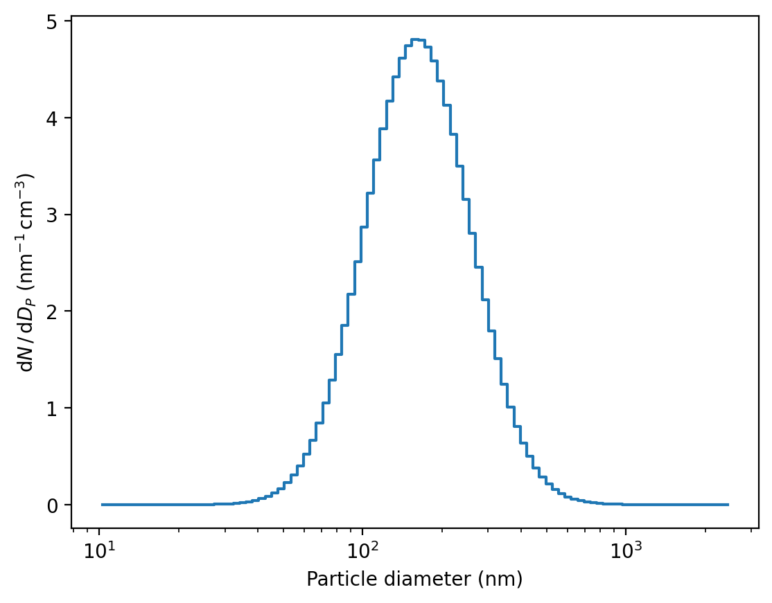
[19]:
sd.plot()
[19]:
(<Figure size 1280x960 with 1 Axes>,
 <Axes: xlabel='Particle diameter (nm)', ylabel='$\\mathrm{d}N\\,/\\,\\mathrm{d}D_{P}$ (nm$^{-1}\\,$cm$^{-3}$)'>)
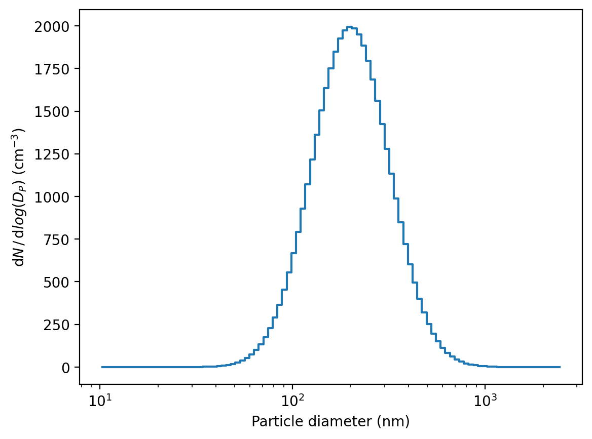
Moment conversion
[31]:
sd = sd.convert2dNdlogDp()
[32]:
sd.plot()
[32]:
(<Figure size 1280x960 with 1 Axes>,
 <Axes: xlabel='Particle diameter (nm)', ylabel='$\\mathrm{d}N\\,/\\,\\mathrm{d}log(D_{P})$ (cm$^{-3}$)'>)
optical properties
Mie
[22]:
sd.optical_properties.parameters.refractive_index = 1.5
sd.optical_properties.parameters.wavelength = 500
sd.optical_properties.extinction_coeff # explore namespace for more Mie results
[22]:
| ext_coeff_m^1 | |
|---|---|
| 0 | 0.000086 |
t-matrix
[33]:
sd.optical_properties.parameters.refractive_index = 1.5
sd.optical_properties.parameters.wavelength = 500
sd.optical_properties.parameters.asphericity = 5
sd.optical_properties.scattering_coeff # explore namespace for more Mie results
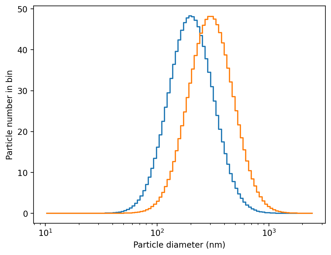
hygroscopic growth
GOTCHA you can loose particles when applying growth!!! See help of sd.grow_sizedistribution function! There are functions that extrapolate size distributions assuming normal distributions. Consider using those.
[85]:
reload(atmsd.hygroscopicity)
reload(atmsd)
[85]:
<module 'atmPy.aerosols.size_distribution.sizedistribution' from '/export/htelg/prog/atm-py/atmPy/aerosols/size_distribution/sizedistribution.py'>
[86]:
sd = atmsd.SizeDist(sd.data, sd.bins, sd.distributionType)
[92]:
sd.hygroscopicity.parameters.kappa = 0.6
sd.hygroscopicity.parameters.RH = 80
[93]:
f,a = sd.plot()
sd.hygroscopicity.grown_size_distribution.plot(ax= a)
/export/htelg/prog/atm-py/atmPy/aerosols/size_distribution/diameter_binning.py:53: NumbaDeprecationWarning: The 'nopython' keyword argument was not supplied to the 'numba.jit' decorator. The implicit default value for this argument is currently False, but it will be changed to True in Numba 0.59.0. See https://numba.readthedocs.io/en/stable/reference/deprecation.html#deprecation-of-object-mode-fall-back-behaviour-when-using-jit for details.
  def match_bins(index, columns, df_match):
/export/htelg/prog/atm-py/atmPy/aerosols/size_distribution/diameter_binning.py:81: NumbaDeprecationWarning: The 'nopython' keyword argument was not supplied to the 'numba.jit' decorator. The implicit default value for this argument is currently False, but it will be changed to True in Numba 0.59.0. See https://numba.readthedocs.io/en/stable/reference/deprecation.html#deprecation-of-object-mode-fall-back-behaviour-when-using-jit for details.
  def match2data(data, df_match,new_data):
[93]:
(<Figure size 1280x960 with 1 Axes>,
 <Axes: xlabel='Particle diameter (nm)', ylabel='Particle number in bin'>)
[ ]: